Next: Numerical Implementation Up: Physical System Previous: Physical System Contents
Wave Forms
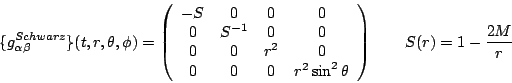
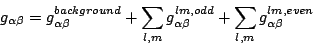
Assume a spacetime
![]() which can be written as a Schwarzschild
background
which can be written as a Schwarzschild
background
![]() with perturbations
with perturbations
![]() :
:
| (part311) |
 |
(part312) |
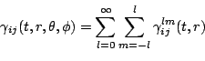
and
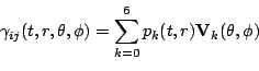
where
| (part313) |
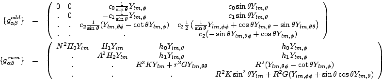
which we can write in an expanded form as
| (part314) | |||
 |
(part315) | ||
| (part316) | |||
 |
(part317) | ||
 |
(part318) | ||
| (part319) |
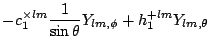
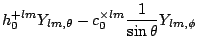
A similar decomposition allows the four gauge components of the 4-metric to be written in terms of three even-parity variables
| (part3110) | |||
| (part3111) | |||
 |
(part3112) | ||
| (part3113) |
Also from
| (part3114) |
where (dropping some superscripts)
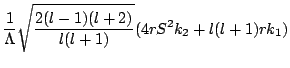
Now, for such a Schwarzschild background we can define two (and only two)
unconstrained gauge invariant quantities
![]() and
and
![]() ,
which from
[10] are
,
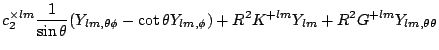
which from
[10] are
![$\displaystyle \sqrt{\frac{2(l+2)!}{(l-2)!}}\left[c_1^{\times lm}
+ \frac{1}{2}\...
...rtial_r c_2^{\times lm} - \frac{2}{r}
c_2^{\times lm}\right)\right] \frac{S}{r}$](img346.png) |
(part3115) | ||
 |
(part3116) | ||
 |
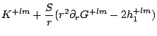
(part3117) |
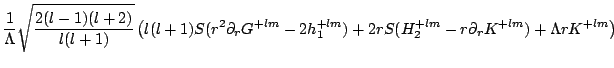
where
 |
(part3118) | ||
![$\displaystyle \frac{1}{2S}
\left[H^{+lm}_2-r\partial_r k_1-\left(1-\frac{M}{rS}...
...1 + S^{1/2}\partial_r
(r^2 S^{1/2} \partial_r G^{+lm}-2S^{1/2}h_1^{+lm})\right]$](img354.png) |
(part3119) | ||
![$\displaystyle \frac{1}{2S}\left[H_2-rK_{,r}-\frac{r-3M}{r-2M}K\right]$](img355.png) |
(part3120) |
NOTE: These quantities compare with those in Moncrief [23] by
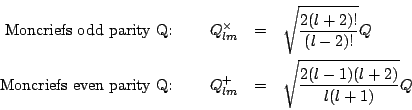
Note that these quantities only depend on the purely spatial Regge-Wheeler functions, and not the gauge parts. (In the Regge-Wheeler and Zerilli gauges, these are just respectively (up to a rescaling) the Regge-Wheeler and Zerilli functions). These quantities satisfy the wave equations
![\begin{eqnarray*}
&&(\partial^2_t-\partial^2_{r^*})Q^\times_{lm}+S\left[\frac{l...
...t)
\right)+\frac{l(l-1)(l+1)(l+2)}{r^2\Lambda}\right]Q^+_{lm}=0
\end{eqnarray*}](img357.png)
where
Next: Numerical Implementation Up: Physical System Previous: Physical System Contents