Time evolution methods provided by MoL

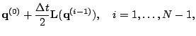
The default method is Iterative Crank-Nicholson. There are many ways of implementing this. The standard "ICN" and "Generic"/"ICN" methods both implement the following, assuming an $N$ iteration method:

$${\bf q}^{(0)} = {\bf q}^{n},$$ (part107)

$${\bf q}^{(i)} = {\bf q}^{(0)} + \frac{\Delta t}{2} {\bf L}({\bf q}^{(i-1)}), \quad i = 1,\dots,N-1,$$ (part108)

$${\bf q}^{(N)} = {\bf q}^{(N-1)} + \Delta t {\bf L}({\bf q}^{(N-1)}),$$ (part109)

$${\bf q}^{n+1} = {\bf q}^{(N)}$$ (part1010)

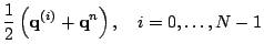
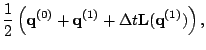
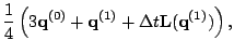
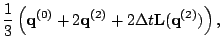
The ``averaging'' ICN method "ICN-avg" instead calculates intermediate steps before averaging:

$${\bf q}^{(0)} = {\bf q}^{n},$$ (part1011)

$$\tilde{{\bf q}}^{(i)} = \frac{1}{2}\left( {\bf q}^{(i)} + {\bf q}^{n} \right), \quad i = 0,\dots,N-1$$ (part1012)

$${\bf q}^{(i)} = {\bf q}^{(0)} + \Delta t {\bf L}(\tilde{{\bf q}}^{(N-1)}),$$ (part1013)

$${\bf q}^{n+1} = {\bf q}^{(N)}$$ (part1014)

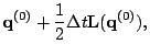
The Runge-Kutta methods are those typically used in hydrodynamics by, e.g., Shu and others -- see [5] for example. Explicitly the first order method is the Euler method:

$${\bf q}^{(0)} = {\bf q}^{n},$$ (part1015)

$${\bf q}^{(1)} = {\bf q}^{(0)} + \Delta t {\bf L}(\tilde{{\bf q}}^{(0)}),$$ (part1016)

$${\bf q}^{n+1} = {\bf q}^{(1)}.$$ (part1017)

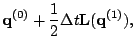
The second order method is:

$${\bf q}^{(0)} = {\bf q}^{n},$$ (part1018)

$${\bf q}^{(1)} = {\bf q}^{(0)} + \Delta t {\bf L} ({\bf q}^{(0)}),$$ (part1019)

$${\bf q}^{(2)} = \frac{1}{2} \left( {\bf q}^{(0)} + {\bf q}^{(1)} + \Delta t {\bf L} ({\bf q}^{(1)}) \right),$$ (part1020)

$${\bf q}^{n+1} = {\bf q}^{(2)}.$$ (part1021)

The third order method is:

$${\bf q}^{(0)} = {\bf q}^{n},$$ (part1022)

$${\bf q}^{(1)} = {\bf q}^{(0)} + \Delta t {\bf L} ({\bf q}^{(0)}),$$ (part1023)

$${\bf q}^{(2)} = \frac{1}{4} \left( 3 {\bf q}^{(0)} + {\bf q}^{(1)} + \Delta t {\bf L} ({\bf q}^{(1)}) \right),$$ (part1024)

$${\bf q}^{(3)} = \frac{1}{3} \left( {\bf q}^{(0)} + 2 {\bf q}^{(2)} + 2 \Delta t {\bf L} ({\bf q}^{(2)}) \right),$$ (part1025)

$${\bf q}^{n+1} = {\bf q}^{(3)}.$$ (part1026)

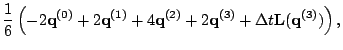
The fourth order method, which is not strictly TVD, is:

$${\bf q}^{(0)} = {\bf q}^{n},$$ (part1027)

$${\bf q}^{(1)} = {\bf q}^{(0)} + \frac{1}{2} \Delta t {\bf L} ({\bf q}^{(0)}),$$ (part1028)

$${\bf q}^{(2)} = {\bf q}^{(0)} + \frac{1}{2} \Delta t {\bf L} ({\bf q}^{(1)}),$$ (part1029)

$${\bf q}^{(3)} = {\bf q}^{(0)} + \Delta t {\bf L} ({\bf q}^{(2)}),$$ (part1030)

$${\bf q}^{(4)} = \frac{1}{6} \left( - 2 {\bf q}^{(0)} + 2 {\bf q}^{(1)} + 4 {\bf q}^{(2)} + 2 {\bf q}^{(3)} + \Delta t{\bf L} ({\bf q}^{(3)}) \right),$$ (part1031)

$${\bf q}^{n+1} = {\bf q}^{(4)}.$$ (part1032)