Purpose

The Method of Lines (MoL) converts a (system of) partial differential equation(s) into an ordinary differential equation containing some spatial differential operator. As an example, consider writing the hyperbolic system of PDE's

$$\partial_t {\bf q} + {\bf A}^i({\bf q}) \partial_i {\bf B}({\bf q}) = {\bf s}({\bf q})$$ (part101)

in the alternative form

$$\partial_t {\bf q} = {\bf L}({\bf q}),$$ (part102)

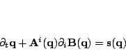
which (assuming a given discretization of space) is an ODE.

Given this separation of the time and space discretizations, well known stable ODE integrators such as Runge-Kutta can be used to do the time integration. This is more modular (allowing for simple extensions to higher order methods), more stable (as instabilities can now only arise from the spatial discretization or the equations themselves) and also avoids the problems of retaining high orders of convergence when coupling different physical models.

MoL can be used for hyperbolic, parabolic and even elliptic problems (although I definitely don't recommend the latter). As it currently stands it is set up for systems of equations in the first order type form of equation (A10.2). If you want to implement a multilevel scheme such as leapfrog it is not obvious to me that MoL is the thing to use. However if you have lots of thorns that you want to interact, for example ADM_BSSN and a hydro code plus maybe EM or a scalar field, and they can easily be written in this sort of form, then you probably want to use MoL.

This thorn is meant to provide a simple interface that will implement the MoL inside Cactus as transparently as possible. It will initially implement only the optimal Runge-Kutta time integrators (which are TVD up to RK3, so suitable for hydro) up to fourth order and iterated Crank Nicholson. All of the interaction with the MoL thorn should occur directly through the scheduler. For example, all synchronization steps should now be possible at the schedule level. This is essential for interacting cleanly with different drivers, especially to make Mesh Refinement work.

For more information on the Method of Lines the most comprehensive references are the works of Jonathan Thornburg [3,4] - see especially section 7.3 of the thesis. From the CFD viewpoint the review of ENO methods by Shu, [5], has some information. For relativistic fluids the paper of Neilsen and Choptuik [6] is also quite good.