Purpose

To demonstrate the use of the Cactus code through a simple, illustrative example.

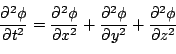
The model problem solved is the 3D scalar wave equation in Cartesian coordinates,

$$\frac{\partial^2 \phi}{\partial t^2} = \frac{\partial^2 \ph... ...2 \phi}{\partial y^2} + \frac{\partial^2 \phi}{\partial z^2}$$

The numerical solution of this equation requires initial data to be specified for

$$\phi(t=0), \qquad \frac{\partial \phi}{\partial t}(t=0)$$

The numerical method employed in these thorns to solve for $\phi$ is a standard 2nd order centered finite difference method. The solution $\phi(t,x,y,z)$ is discretised using

$$\phi(t_i,x_i,y_i,z_i) = \phi^n_{i,j,k}$$

where, for example,

$$x_i = x_0 + i \Delta x$$

The solution at any timeslice can then be found iteratively using the previous two timeslices using the algorithm

$$\phi^{n+1} = 2(1- \rho_x^2 - \rho_y^2 - \rho_z^2) \phi^n_{i,j,k} -\phi^{n-1}_{i,j,k} + \rho_x^2(\phi^n_{i+1,j,k}-\phi^n_{i-1,j,k})$$

$$+ \rho_y^2(\phi^n_{i,j+1,k}-\phi^n_{i,j-1,k}) + \rho_z^2(\phi^n_{i,j,k+1}-\phi^n_{i,j,k-1})$$ (part1061)

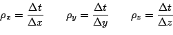
where we define the Courant factors

$$\rho_x = \frac{\Delta t}{\Delta x} \qquad \rho_y = \frac{\Delta t}{\Delta y} \qquad \rho_z = \frac{\Delta t}{\Delta z}$$